Recently, my paper Remaining cycle time prediction: Temporal loss functions and prediction consistency got accepted for publication in Nordic Machine Intelligence (NMI). The paper addresses the issue of improving the performance from the so-called earliness aspect by introducing a temporally-weighted penalty to the loss function.
Earliness refers to how well the model predicts remaining time, early in a sequence of events (a business process instance such as a ticket in customer service). Earliness is often desirable, as it gives the process manager the most time to react when it is needed.
The main idea of this paper was thereby to see if this performance aspect could be improved by changing the loss function used in the best performing approach at the time (https://arxiv.org/abs/1711.03822).
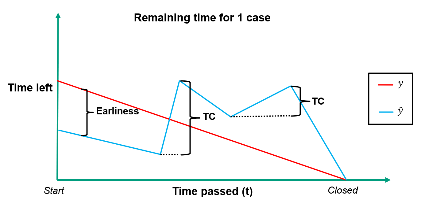
The illustration above shows the actual remaining time \(y\) and the predicted remaining time \(\hat{y}\) for a single imagined customer service case. The earliness perspective is shown as the distance between the actual and predicted values in the beginning, and the TC perspective (introduced later) shows the increases in predicted remaining time.
Tested loss functions
To evaluate the effect of focusing the learning effort on the early part of the sequences via a temporal penalty, three loss candidates were tested alongside the baseline loss which is most commonly used in previous studies.
Baseline loss: Mean absolute error (MAE)
\(MAE = \frac{1}{N}\sum_{i=1}^{N}\frac{1}{T}\sum_{t=1}^{T_i}\mid y_{t}^i - \hat{y}_{t}^i\mid\\\)
Candidate 1: MAE with Exponential temporal decay
\(MAE_{EtD} = \frac{1}{N}\sum_{i=1}^{N}\frac{1}{T}\sum_{t=1}^{T_i} \mid y_{t}^i - \hat{y}_{t}^i\mid + \frac{\mid y_{t}^i - \hat{y}_{t}^i\mid}{e^{\left(t\right)}}\\\)
Candidate 2: MAE with Power temporal decay
\(MAE_{PtD} = \frac{1}{N}\sum_{i=1}^{N}\frac{1}{T}\sum_{t=1}^{T_i} \mid y_{t}^i - \hat{y}_{t}^i\mid + \mid y_{t}^i - \hat{y}_{t}^i\mid ^{\frac{T_i-t}{T_i}}\\\)
Candidate 3: MAE with Moderate temporal decay
\(MAE_{MtD} = \frac{1}{N}\sum_{i=1}^{N}\frac{1}{T}\sum_{t=1}^{T_i} \mid y_{t}^i - \hat{y}_{t}^i\mid + \frac{\mid y_{t}^i - \hat{y}_{t}^i\mid}{t}\\\)
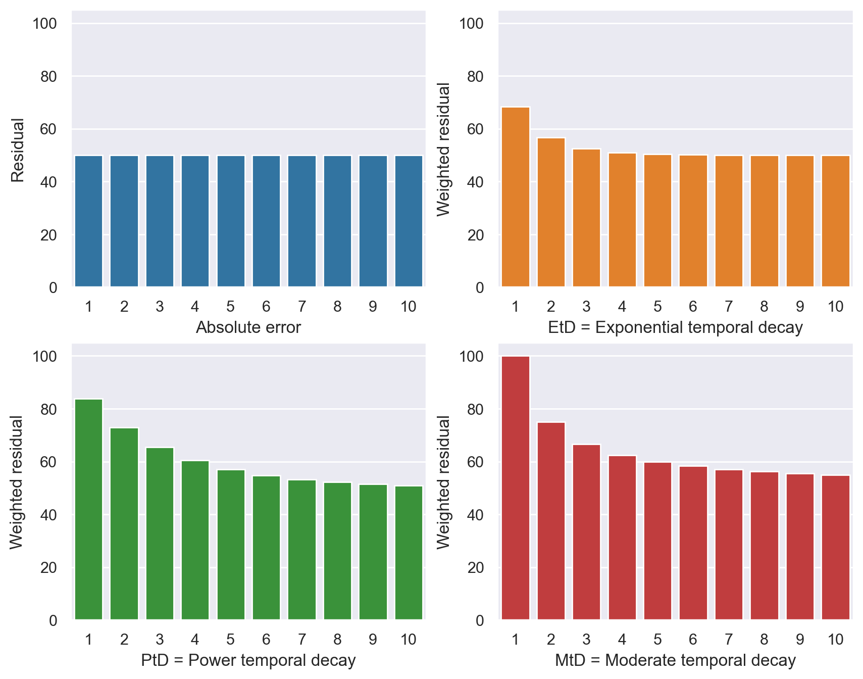
Essentially these variants vary in terms of their slope, which can be seen by the figure below. In this example we have an error of 50 units at each time step, and the size of the bars thereby show how the loss function penalizes that constant error. E.g. \(MAE_{MtD}\) weight the error at t=1 to be twice as high as the baseline \(MAE\), while it approaches 50 as \(t\rightarrow\inf\) at a faster rate than \(MAE_{PtD}\).
Temporal consistency
Another aspect of this paper was the evaluation part, in which I introduce a new metric for model assessment. The idea here is that the ideal remaining time model represents time in a monotonically decreasing manner (remaining time does not increase - time only moves in one direction).
One can of course say that it is unrealistic to create a model that will not have this type of behaviour, or that an operational model should be able to correct itself - which are both valid arguments. However, this does not mean that we should not strive to try and reduce this behaviour as much as possible. The more often the direction of an estimate is changed, the less useful the model becomes, especially for planning.
The proposed Temporal Consistency measure is thereby intended for the practicioner (Data scientist) to use for model evaluation, such that end-users will know to which degree this might become a problem out of sample.
\(TC = \frac{1}{N}\sum_{i=1}^{N}\frac{1}{T-1}\sum_{t=2}^{T_i} H\left( \hat{y}_{t}^i - \hat{y}_{t-1}^i\right)\mid\hat{y}_{t}^i - \hat{y}_{t-1}^i\mid\\\)
where
\(H(x)=
\begin{cases}
1, & x\geq 0\\
0, & x < 0
\end{cases}
\\\)
The TC only measures when the predicted remaining time between two time steps (activities in a process) increases. As seen from its formulation, it also only measures the differences between the predictions. It should therefore be seen as an addition to other model selection metrics, such as mean absolute error, etc.
Experiments, Results, and Conclusion
If you have read this far and remain interested, I strongly recommend reading the full paper: https://journals.uio.no/NMI/article/view/10141. In brief, it was found that the loss modifications led to small but significant improvements in terms of model earliness performance on out-of-sample data. Interestingly, they did not improve performance from the TC perspective.
I plan to do a follow-up study to further explore these results via Monte Carlo simulation.